It must be emphasized that our discussion of general equilibrium prices GEP takes place here, among the criteria for economic stasis, rather than among the operational devices we posit as controlling economic order. SFEcon's operational hypotheses, being dynamic, tolerate no references in equilibrium. The calculations set forth below are only used to initiate models in a state of general optimality; and they only serve a theoretical discussion by partly describing the state to which a model subsides when its parameters are held constant. SFEcon's notions about general price equilibria should be familiar except for 1) their reliance on our matrix structure and 2) their novel consideration of the interest rate -i_K.

Source code and sample data for SFEcon’s GEP algorithm can be found in either of two MSWin Excel exemplars for Model 0:  M0.3.2.1 or M0.3.2.3. These models operate on a 5x5 input/output array composed of three generic industrial sectors and two households. As shown in Figure 1, the generic sectors 1, 2, and 3 respectively produce capital, general, and non-durable goods. The two household sectors L and N respectively represent a bourgeoisie and a proletariat. (A separate .pdf illustration of the figures in this segment is likely to prove helpful.)

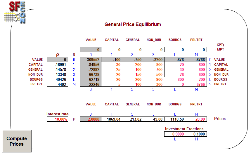
Fig. 1

The data that must given to SFEcon’s GPE algorithm are shown in red (not maroon). As indicated, physical input/output data comprise most of the data to be honored in the determination of prices. For the purposes of this mathematical development, R_IJ is the physical rate at which a sector I employs a commodity J. Our algorithm presumes a physical equilibrium in which factor employments are just sufficient to produce a vector of commodity outputs -R_0J that exactly replaces everything being used to create the next generation of goods. R₀₂ = -750 means that the general goods sector 2 produces/sells just enough output to replace assets being used at rates of 200 + 100 + 150 + 200 + 100 physical units per year.

Following conventional practice, these data are used to construct a matrix equation that brings our unknown vector of commodity prices P_J into a formulation of the sectors’ profits. Figure 2 expresses profits in matrix form: each sector I’s sales P_IY_I are subtracted from its cost of sales SP_JR_IJ to compute earnings in the negative sense required by SFEcon’s sign convention. A continuation of normal practice would presume that normal profits are somehow expressed in the cost of sales, and then equate the expression in Figure 2 to a null vector representing zero extraordinary profits. Solving this system would require specification of one price to determine the general price level, which would then enable solution of the entire system via Gaussian elimination.

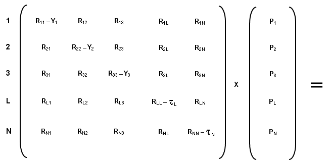
Fig. 2

The SFEcon system is more complicated because profits are made explicit. Our GEP algorithm operates to generate a profits profile r in which earnings of the industrial sectors 1, 2, and 3 will exactly offset interest incomes of the household sectors L and N. In the example of Figure 1, r expresses industrial profits of 16991 + 14578 + 13348 $/year that are exactly absorbed as passive household incomes of 40426 + 4492 $/year.

Formulation of the profits profile r begins by presuming that all of the money flowing through the generic industrial sectors must generate a return at the prevailing interest rate -i. Note that an interest rate of -i = 10% has been recorded among Figure 1’s input data. As shown in the first three elements of Figure 3, the return required on an industrial sector’s operations is given by the interest rate -i times the value of the sector’s asset turnover.

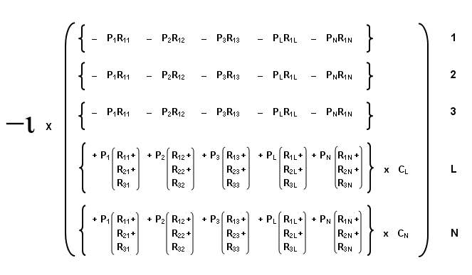
Fig. 3

Since Model 0 permits only one financial intermediary, his portfolio must include the assets of all industrial sectors; and his function is to channel all sectors’ earnings to the household sectors in proportion to their holdings of his universal mutual fund. Initiation of models having more than one household sector requires specification of the households’ relative shares in ownership of the economy’s earning assets. Figure 1 has these data recorded as ‘Investment Fractions’: the bourgeoisie sector L is initially given 90% ownership of the economy’s assets, leaving 10% for the proletariat. These factors, C_L and C_N are applied to earnings from the intermediary’s portfolio in elements of L and N of Figure 3. Relative and absolute fortunes of the households are of course free to change in the dynamic operations of Model 0.

Figure 3’s expression of the profits profile r provides a right-hand-side with which to complete Figure 2’s development of the earnings equation’s left-hand-side. Inspection shows that the 6x1 vector of Figure 3 allows a factoring-out of the price vector to leave a {5x5}x{5x1} system that is congruent with Figure 2. Subtracting the right side of this system from the left will leave a complicated {5x5} coefficients matrix times a {5x1} prices vector equaling a {5x1} null vector on right side. Solving this system then requires exterior specification of one price, which Figure 1 is seen to request in terms of the proletarian wage of $20 per hour.

SFEcon’s price vector is completed by exterior specification of the money price P₀ $/G for one unit of absolute value G. This price does not bear upon the GPE algorithm in any way. It serves only to determine number of absolute value units to be made available at a model’s initiation. P₀ is used to compute the sectors’ initial absolute values of asset turnover from their monetary turnover rates as computed via the money prices. A model’s initial total number of value units represents all the sectors’ initial asset values. This total is not allowed to change during a model’s operation; but value does flow among the sectors to reflect their changing fortunes. Development of SFEcon’s notions on the value question will proceed with another, later discussion of price formation in a dynamic context.